Activity 18 - Noise model and basic image restoration

Several factors affect the quality of a digital image. For one, the lenses of the camera, especially for single-lens cameras, distort the captured image. In our previous activity, we performed image processing techniques to correct such distortions. Aside from distortion, noise which is random variation of brightness and color information of images[2], also cause undesirable degradation to the captured image that usually arises during acquisition. For instance, temperature which alters the response of a camera sensor affects the amount of noise in an image[1]. In restoring such images, we use our knowledge of the degradation phenomenon, model it and perform an inverse process in order to recover the image.

Noise are composed of random variables characterized by certain probability distribution function (PDF)[1]. In this activity, we explore on most common noise models found in image processing applications as well as some basic noise-reduction filters used in image restoration.

Noise Models

Gaussian noise:

p(z) = (¹/√ _2πσ )e^{-(z-μ)2/_2σ2}

Rayleigh noise:

p(z) = (²/_b)(z - a)e^-(z-a)2/_b for z > a else p(z) = 0

Erlang (Gamma) Noise:

p(z) = [^abzb-1/_(b-1)!] e^-az for z > a else p(z) = 0

Exponential Noise:

p(z) = ae^-az for z > a else p(z) = 0

Uniform Noise:

p(z) = ¹/_(b-a) if a < z < b else p(z) = 0

Impulse (salt an pepper) Noise:

p(z) = P_a for z = a
p(z) = P_b for z = b
p(z) = 0 otherwise

The figure below demonstrates the effect of each noise PDF to an image. Here we initially observe a grainy effect of the noise.

Figure 1. (left) Original image and (right) the image added with (clockwise from upper left) Gaussian, gamma, exponential, Rayleigh, uniform and, salt&pepper noise.

From the original grayscale value histogram of the image (shown in Figure 2), upon application of the noise to the image, the histogram was transformed as in Figure 3.

Figure 2. Grayscale value histogram of the image

Figure 3. Histogram of grayscale values from the generated noisy images: (clockwise from upper left) Gaussian, gamma, exponential, Rayleigh, uniform and, salt&pepper noise.

Basic noise-reduction filters

These filters takes a window S_xy in an image with center x,y and perform averaging.
Arithmetic mean filter (AMF)

Geometric mean filter (GMF)

Harmonic mean filter (HMF)

Contraharmonic mean filter (CMF)

CMF is good in removing salt&pepper noise. If Q>0, it removes pepper noise. If Q<0, it removes salt noise.

Restoration

We have tested the effect of the window size to the quality of the reconstructed image. The figure below shows the reconstructed images using the four filters for sizes of S_xy = {3x3, 5x5, 9x9}. We observe that smaller window size resulted to a relatively grainy restoration than with that of larger window size. On the other hand, large window size resulted to a more blurry image. In the following reconstructions, we used a window size of 5x5.

Figure 4. Reconstructed image of Gaussian-noised image using (from top to bottom) AMF, GMF, HMF and CMF (Q= 1) at different window sizes (left to right) 3x3, 5x5, 9x9.

Here we show the effects of the filters to the noised images.

Figure 5. (right)Reconstruction of (left)noisy images: (top to bottom) Gaussian, gamma, exponential, Rayleigh, uniform and, salt&pepper noise using (from 2^nd column to the right) AMF, GMF, HMF and CMF (Q=1).

From Fig. 5, we see that for all noised images, the AMF produced a consistent results although may not be the best result. This technique can thus be use generically for noisy images. GMF also produced a very good restoration for all noised images except for the salt&pepper-noised image. HMF is also resulted to a good reconstruction except for Guassian and salt&pepper-noised images. CMF (Q= 1) produced a good result except for exponential and salt&pepper-noised image. Salt&pepper-noised image was harder to restore compared to others. Moreover, we see that CMF (Q=1) was not able to correctly restore a salt&pepper-noised image, as previously said. Now we demonstrate the effect of CMF to salt-only and pepper-only-noised image.

Figure 6. Image reconstruction of Q = 1 and Q= -1 CMF for (top to bottom) the image with salt and pepper, salt-only and pepper-only noise. CMF cannot properly reconstruct a salt& pepper-noised image. Salt is removed when Q is negative. Pepper is removed when Q is positive.

We indeed see that CMF can perfectly restore images with salt noise and pepper noise alone.

Figure 7. Test image taken from [3]

Below are reconstructions of noised images using (from upperleft clockwise) AMF, GMF, CMF, and HMF.

Figure8. Reconstruction of a Gaussian-noised image.


Figure 9. Reconstruction of a gamma-noised image.


Figure 10. Reconstruction of a exponential-noised image.


Figure 11. Reconstruction of a Rayleigh-noised image.


Figure 12. Reconstruction of a uniform-noised image.


Figure 13. Reconstruction of a salt&pepper-noised image.

In this activity, I give myself a grade of 10 for finishing it well.
I thank Irene, Janno, Martin, Master, Cherry for the help.

References:
[1] AP186 Activity 18 manual
[2] http://en.wikipedia.org/wiki/Image_noise
[3] http://bluecandy.typepad.com/.a/

Activity 17 - Photometric Stereo

Objects appear different depending on where the light source illuminating it is located. Shadows form at different locations. In this activity, we demonstrate a shadow model and extract shape from the shadows. Models depend on the type light source (point source, line source, etc.) used and where the light source is located. One of the more simple model is when the light source is placed at infinity. In general, when the light source is nearby, the brightness of an object illuminated by it is given by:

B(P) = [ρ(P)n(P)•S(P)]/R(P)²

where B(P) is the brightness of the object, S(P) is a vector from the light source and R(P) is the distance of the light source from the object.
In an infinite light source, 1/r dependence of B(P) disappears and the vector S(P) becomes constant for every point in the object. Thus the equation becomes:

B(P) = ρ(P)n(P)•S_o

In capturing an image of an object, we assume that it is proportional to the brightness of the object:

I(x,y) = kB(x,y) = kρ(x,y)n(x,y)•S_o = g(x,y)•V_o

where g(x,y) = ρ(x,y)n(x,y) and V_o=kS_o.

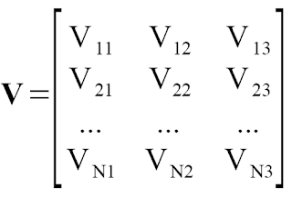
When an object is illuminated by light N light sources, Vo takes the form:

Each row represents the position (x,y,z) of the source in 3D space. Given an image with its intensity equal to its grayscale value, we can determine g(x,y) using the equation above. If we took a N captures of the surface of object illuminated by N light sources, then for each point (x,y):

I₁(x,y) = V₁₁g₁ + V₁₂g₂ + V₁₃g₃
I₂(x,y) = V₂₁g₁ + V₂₂g₂ + V₂₃g₃
I_N(x,y) = V_N1g₁ + V_N2g₂ + V_N3g₃

or in matrix form:

I = gV

Since we know I and V, we can calculate g using:

g = (V^TV)^-1VI

The normal vector can be solved by:

To get the surface elevation of point (u,v) on the surface, we use:

where

In this activity, we captured four images of a hemisphere illuminated by a far away light source located at four positions V:

(0.085832, 0.17365, 0.98106)
(0.085832, -0.17365, 0.98106)
(0.173650, 0.0, 0.98481)
(0.163180, -0.34202, 0.92542)

Below are the images taken for each light source locations.

Figure 1. Images of a hemispheres illuminated by a light source located at different positions

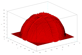
Using the procedure above, we obtained a 3D image of the surface shown in Fig.2.

Figure 2. 3D reconstruction of the hemisphere

Here, we have successfully reconstructed the image. The reconstruction, however, is not smooth. Some parts do not follow the contour of a hemisphere.

In this activity, I give myself a grade of 10 for a successful reconstruction of the surface.

I thank Irene, Alva, Orly for very very useful help. :)

Activity 16 - Neural Networks

In the previous activities, we have used Euclidean distance and LDA as classifiers for pattern recognition. In this activity, we tried the neural networks. A neural network is a computational model of how neurons in the brain works. Basically, just as the brain does pattern recognition, the neural network is fed with features of known patterns; in which case, it "learns" the rules for classification from the input it receives.
Just as the neurons pass electrical signals to other neurons, this model (McCoulloch, Pitts 1943) essentially works the same way. With input signals x_i, (see Fig.1) a neuron receives weighted inputs(w_i*x_i) and lets the sum of all the signal it receives act on an activation function g. The resulting signal z is then passed to other neurons[1].

Figure 1. Artificial neuron

The same process takes place as the signal is passed from neuron to neuron. This network of neurons is called the neural network.

Figure 2. Neural Network

The neural network is composed of an input layer, a hidden layer, and the output layer. The input layer receives the signal (features) which is passed onto the hidden layer. The hidden layer then passes it to the output layer[1].

Results

Using a code originally written by J. Tugaff [2], we use neural network to classify objects as 1-peso coin, 25-cents coin, long leaf, short leaf or flower using r-g chromaticity and dimension ratio (length/width) as features. (Code needs modification depending on the number of classes and features used.)

Learning process
As training , we used the features of 5 samples/class as inputs to the neural network. It is trained such that it outputs: [1 0 0 0 0] for 1-peso coin, [0 1 0 0 0] for 25-cents coin and so on.

Figure 3. Plot of the distinguishing capability of the neural network with (left) learning rate and (right) training cycles T.

Before the classification, we checked the distinguishing capability (the ability to properly separate classification from other classes)of the neural network as a function of the learning rate and training cycles T. We checked it by using the training set as our test set. We took the average value of the "supposedly 1" outputs. Fig.3(left) shows the average against learning rate. An increasing trend is observed. As learning rate increases, the output approaches to 1 thus the network is able to classify the objects properly. We also observed an increasing trend when T increases. High T improves learning process resulting to better classification.
Based on these results, it is quite a good idea to choose learning rate and T as high as possible. However, this is very time-consuming to do. This will slow down the learning process which makes it impractical.¹ For our case, we use T = 5000 and learning rate = 1 for training.

After training, we tested the training set to verify that the network has "learned". The result of classification is summarized on the table below.

Table 1. Classification of the training set used in the learning process of the neural network.

Here we see that the network is able to identify properly identified the training set hence the network has already learned, we can now use it to classify our test objects.

Classification of test objects
In the table below, we show the result of classification of the test objects. Here, we have achieved a 96% correct classification.

Table 2. Classification of test objects using the neural network

¹ If one, on the other hand, is willing to wait for better results, he might as well choose higher learning rate and T.

I thank Master, Kaye and Thirdy and Irene for very useful help.

I give myself a grade of 10 for doing a good job.

References:
[1] Applied Physics 186 Activity 16 manual
[2] http://cole-ap186.blogspot.com/

Activity 15 - Probabilistic Classification

In the previous activity, we tried to classify objects into classes based on a set of features that describe the objects. Particularly, we used the Euclidean distance as a classifier for our dataset. In this activity, on the other hand, we use another classifier called the Linear Discriminant Analysis (LDA). Discriminant analysis is a statistical approach in pattern recognition. LDA assumes that the classes of objects are linearly separable (as the term linear applies)-- meaning, the classes of objects can be separated by linear combination of features that describe the object[1]. The LDA formula is given by:

f_i = u_iC^-1x_k^T - 1/2u_iC^-1u_i^T + ln(p_i) .

where u_i is the mean features of the class i, C is the covariance matrix obtained from the training set, x_k is the features of test k^th test object, and p_i is the prior probability of a class i.

Mean Features of a Class

Given features of a set of test objects of the classes 1 and 2, (in this case, we have 3 test objects and 2 features for class 1)

x₁ = [a_o b_o; a₁ b₁; a₂ b₂] and x₂ = [c_o d_o; c₁ d₁]

mean feature of class 1 is calculated as:

u₁ = [mean(a_o,a₁,a₂) mean(b_o,b₁,b₂)]

Covariance Matrix
From the features of the whole training set (contains all training samples of all classes), one can calculate the global mean vector. This is essentially the mean features of the whole training set.
For example, given a data set

x = [a_o b_o; a₁ b₁; a₂ b₂; c_o d_o; c₁ d₂] ,

the global mean vector is given by

u = [mean(a_o,a₁,a₂,c_o,c₁) mean(b_o,b₁,b₂,d_o,d₁)]

From the u, we can solve the mean corrected data x_i^o for each class i

x_i^o = x_i -u .

The covariance matrix of a class i is:

c_i = [(x_i^o)^Tx_i^o]/n_i

where n_i is the number of test samples used for class i.
The covariance matrix of the whole test set is then solved using:

C = 1/n Σ n_i⋅c_i

where n is the number of samples in the whole data set.

Prior Probability

The prior probability of class i is given by:

p_i = n_i/n .

Results

We used the LDA formula in classifying objects in our data set. The object k is classified as belonging to class i if it resulted the highest f at i. Below is the result of our classification. Highlighted values are the maximum f_i obtained per sample. Samples are classified according to i where highlighted values occur.

Table 1. LDA results of 5 test samples of 1-peso coins,25-cent coins, long leaves, short leaves and flowers.

Based on the table, we were able to get a 92% classification of objects.

In this activity, I give myself a grade of 10 for understanding ang implementing properly LDA.

I thank Mark Jayson and Luis for happy conversations while doing the activity in the IPL lab.

References:
[1]http://people.revoledu.com/kardi/tutorial/LDA/Numerical%20Example.html