In this activity, we are tasked to perform restoration algorithm to motion blurred images with additive noise.
Model
Degradation process is modeled as a degradation function (see figure below), together with an additive noise, applied to an input image.

The blurring process is taken as the convolution of the degradation function h(x,y) with the input image f(x,y). With the addition of noise, the output image becomes:
g(x,y) = h(x,y)*f(x,y) + η(x,y)
G(u,v) = H(u,v)F(u,v) + N(u,v)


We take the Fourier transform (FT) of the output function which results to a simple algebraic form:
Now, the degradation transfer function H(u,v) is given by:
H(u,v) =[T/π(ua+vb)] sin [π(ua+vb)]e-jπ(ua+vb)where a,b are the displacement of the image along the x and y direction, T is the exposure time of the capture (shutter speed).
Below is an example of an blurred image (a = 0.1, b = 0.1, T = 1) with an additional Gaussian noise (μ = 0.01,σ = 0.001).
In restoring blurred images, we use the Minimum square error (Weiner) filtering. This technique incorporates the degradation function (blurring process) and the noise to reconstruct a corrupted image (f) and finding an estimate f ^ such that, as the name implies, the mean square error between them is minimum. The best estimate of the image in the frequency domain is given by:

where Sη = |N(u,v)|2 (power spectrum of the noise) and Sf = |F(u,v)|2 (power spectrum of the undergraded image).
Using the above equation, we demonstrate the following restorations at various exposure times (T) and motion blur displacements (a,b).
Using the above equation, we demonstrate the following restorations at various exposure times (T) and motion blur displacements (a,b).
Figure 2. Restored images (down) increasing motion displacements a = b = 0.01, 0.1, 1 and (from left) increasing T (0.1, 1, 5, 10 and 50).
From the figure, we observed that increasing T results to a better restoration of the image. As previously mentioned, T is the exposure time of capture. It measures the amount of light coming into the sensor of an imaging device. This is the reason why we notice that images using small T tend to be relatively darker than when using larger T. Moreover, T also affects how movements appear in a picture[2]. Less Ts are intended for freeze fast moving objects, such as in sports. High Ts, on the other hand, are intended for intentional blurring of images for artistic purposes[2]. Our results suggest that higher T renders better image restoration. At these values, we gain more information of the blurring process; thus we are able to have improved estimate of the original image.
Also, as seen from the figure, the quality of the restored image decreases with increasing motion blur displacements. As expected, increasing the values of a and b enhance the blur resulting to an inevitably poor restoration of the image.
Most of the time, given an image regardless as being blurred or not, we do not have an idea of the distribution of the noise contained in that image. Hence, the equation above cannot be solved if we do not know the power spectrum of the noise. We thus approximate the equation by replacing the last term of the denominator with a specified constant K (shown below).

We explored on the effect of the value of K to the quality of the restoration. The figure below shows the restored images as K varies. As seen, the restoration quality decreases with K. From the equation above, K replaces the ratio Sη/Sf (the ration of the spectrum of noise and the spectrum of the undergraded image). K determines the relative degree of noise with respect to the image. The choice of higher values of K comes with the assumption that the image contains a high degree of noise. Hence, increased K (K higher than the actual Sη/Sf) implies lesser possibility of rendering a good result.

Figure 3. Restored images (down) increasing motion displacements a = b = 0.01, 0.1, 1 and (from left) increasing K (0.00001, 0.001, 0.1, and 10).
Note: Most of the results presented were qualitatively described i.e, the qualification of a good or bad quality of the images is subjective. A better and meaningful presentation of the results is to take the Linfoot's criterion (FCQ) as a qualifier and plot it with the parameters a,b, K and T.
In this activity, I give myself a grade of 10 for performing the activity well.
I thank Kaye, Irene and Mark Jayson for useful discussions.
References:
[1] Applied Physics 186 Activity 19 manual
[2] http://en.wikipedia.org/wiki/Shutter_speed
[3] http://www.smashingapps.com/wp-content/uploads/2009/04/grayscale-technique.jpg
[1] Applied Physics 186 Activity 19 manual
[2] http://en.wikipedia.org/wiki/Shutter_speed
[3] http://www.smashingapps.com/wp-content/uploads/2009/04/grayscale-technique.jpg


