In this activity, we were tasked to get a poor-contrast grayscale image from the web. Using the histogram manipulation technique, the goal is to make a high-contrast image out of the original image.
In histogram manipulation, the first step is to take a histogram of the pixel values in the image (histogram is plotted with pixel values on the x-axis and frequency of occurrence of the pixel value on the y-axis. The histogram gives an idea of how many of a pixel value is contained in the image. Once the histogram is made, a cumulative distribution function (CDF) can be plotted. CDF is just the cumulative sum of the values on the y-axis plotted with pixel values. (It is better to work with CDF than histogram as we would see later.)
In histogram manipulation, the first step is to take a histogram of the pixel values in the image (histogram is plotted with pixel values on the x-axis and frequency of occurrence of the pixel value on the y-axis. The histogram gives an idea of how many of a pixel value is contained in the image. Once the histogram is made, a cumulative distribution function (CDF) can be plotted. CDF is just the cumulative sum of the values on the y-axis plotted with pixel values. (It is better to work with CDF than histogram as we would see later.)
To start with, below is the graysacle image taken from the web.

Figure 1. Grayscale image taken from http://homepages.inf.ed.ac.uk/rbf/HIPR2/images/wom1.gif. The figure is then converted to a jpeg file.
Using Scilab, the histogram, as well as the CDF as shown below, of the image in Fig.1 was obtained.


Figure 2. (above) Histogram and (below) CDF of the image in Fig. 1.
As observed from the plots in Fig.2, the CDF is cleaner to see than the histogram. Having the advantage, CDF is easier to manipulate than the histogram.
In histogram manipulation, a desired CDF is needed. This will be used to alter the pixel values contained in the original image. The method is illustrated below.
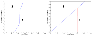
Figure 3. Data manipulation procedure
The desired CDF is of a uniform distribution.
Performing this procedure for all pixel values (0-255), a reconstructed image shown below was obtained.

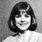
Figure 4. Reconstructed image
Figure 5. (above) Histogram and (below) CDF of the reconstructed image.
In histogram manipulation, a desired CDF is needed. This will be used to alter the pixel values contained in the original image. The method is illustrated below.

Figure 3. Data manipulation procedure
The desired CDF is of a uniform distribution.
Data manipulation procedure done in the following:
(Step 1) Take a pixel value from the CDF of the image in Fig.1
(Step 2) Obtain the value on the y-axis corresponding to the pixel value
(Step 3) Project the y-axis value onto the desired CDF
(Step 4) Take the pixel value from the desired CDF corresponding to the y-axis value.
The pixel value in the image is then replaced by the pixel value from the desired CDF.
The code implementation for a linear desired CDF is written below:
h1 = zeros(256,256);
for i=0:255
new = m(i+1)*255;
h1 = h1 + (im == i)*new;

Figure 4. Reconstructed image
As seen, the image highly contrasted compared to the previous image as a result of the procedure. We also characterize the image by taking its pixel histogram and CDF.


Figure 5. (above) Histogram and (below) CDF of the reconstructed image.
The histogram of the reconstructed image is different from the original image. It is also interesting to note that the spread of the histogram of the reconstructed image is larger than that of the original image indicative of the high contrast of the reconstructed image. Moreover, looking at the CDF of the reconstructed image, it resembles a straight line closer to the desired CDF.
To further explore the technique, a desired CDF that mimics the nonlinear response of the human eye was used. Below is the desired CDF used in reconstructing the image.
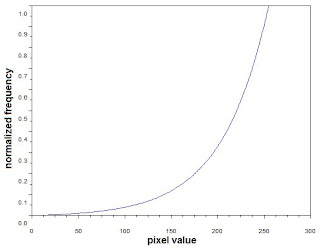
Figure 6. Exponential CDF used in reconstructing the image

Figure 7. Reconstructed image using a nonlinear desired CDF
Compared to the previous reconstruction, the image in Fig.1 is brighter (many of the pixel have high values). we can readily attribute this to the desired CDF used. The latter favors high-valued pixels. As a result, a bright reconstructed image was obtained.
Figure 8. (above) Histogram and (below) CDF of the reconstructed image using nonlinear desired CDF
It can also be seen from Fig. 8 that the histogram of the constructed image has high amplitudes on high-value pixels which indicates a bright image. Also the CDF of the reconstructed image followed the desired CDF.
In this work, i will give myself a grade of 10 for doing it right. Good job for myself.
To further explore the technique, a desired CDF that mimics the nonlinear response of the human eye was used. Below is the desired CDF used in reconstructing the image.

Figure 6. Exponential CDF used in reconstructing the image
The same procedure was done as before and a reconstructed image shown below was obtained.
The code implementation for a nonlinear desired CDF is written below:
h1 = zeros(256,256);
for i=0:255
new = int(50*log(m(i+1)*(exp(255/50)-1)+1));
h1 = h1 + (im == i)*new;
The code implementation for a nonlinear desired CDF is written below:
h1 = zeros(256,256);
for i=0:255
new = int(50*log(m(i+1)*(exp(255/50)-1)+1));
h1 = h1 + (im == i)*new;

Figure 7. Reconstructed image using a nonlinear desired CDF


Figure 8. (above) Histogram and (below) CDF of the reconstructed image using nonlinear desired CDF
It can also be seen from Fig. 8 that the histogram of the constructed image has high amplitudes on high-value pixels which indicates a bright image. Also the CDF of the reconstructed image followed the desired CDF.
In this work, i will give myself a grade of 10 for doing it right. Good job for myself.


