Activity 14 - Pattern recognition

The human brain has the capacity to discriminate from one object to another. From the stigma it receives from the eyes (-or from other sensory organs), one of the things that human does is to find significant features unique to the objects and draw,as well, overlapping features between different objects that will allow to recognize things. The aim of computer vision is to approximate the pattern recognition capabilities of the human brain. Various features can be found in a certain object or pattern -- color, size, shape, area, etc. We use such features to identify an object as a member of a set that has the same properties (this set is called a class).
In this activity, we are tasked to classify objects according to their classes using their physical features. We should be able to (1) find the correct features that will effectively separate the classes and (2) create a classifier (or an algorithm) that is suitable for the task.

In Task 1, we determine the useful features and train a representative set of objects of known class and calculate the feature values (for example, area). An average value per feature is taken from the whole class.

where m_j is the average for all feature x_j of class w_j. It is a 1xn matrix for all features n. These average values will be used as the basis for classification. In our case, we used the r-g chromaticity (discussed in Activity 12)and dimension ratio (length/width) as features for the set of classes we gathered (image is shown below).

Figure 1. Dataset of classes used that contains a set of short and long leaves, flowers, and 25-cent and 1-peso coins.

Once the m_j for all the classes are done, we are now ready to classify a test object based on its features. We extract all the needed features x and determine what class it belongs to. For Task 2, we used the Euclidean distance as a classifier for our test objects. It is given by:

d_j(x) = x^Tm_j - 1/2 m_j^Tm_j

This determines how close the features x of an object to the features of class j. The object will be classified as belonging to a class which yields the largest d_j.

Results

Below is 3D plot of features extracted from the objects in our dataset. We readily see an obvious separation of class clusters of the leaves (short and long) and of the flowers. One reason is that the color of the flower is different from the color of the leaves. The difference in the dimension ratio of the short leaves and long leaves has also separated the two leaf types. However, class clusters of the coins were not well separated. Based on the criteria used, the dimension ratio cannot possibly separate the two since both are circular (dimention ratio ~ 1). Only the color determined by the r-g chromaticities will be able to separate them.

Figure 2. Separation of class clusters using the r, g and dimension ratio as features

We take a look at the distribution of points using only the r-g chromaticities -- Fig.1 as viewed from the above. Here, we see that there is an overlap between the clusters of 1-peso and 25-cent coins. In r-g chromaticity diagram (see Fig. 3 in Activity 12), the color yellow and white, which are the colors of the 25-cents and 1-peso, respectively, lie close to each other. It is thus expected that the clusters be consequently close. The overlap is caused by the highly reflective surface of the coins. In our case, a 25-cent coin is misidentified as a 1-peso coin. Highly reflective 25-cents (the new ones) will appear as though it is a 1-peso coin.

Figure 3. r-g chromaticities of the samples. A single data point overlap of the between two clouds of data points -- cloud of peso coins (inverted triangle) and 25 centavo coins (filled diamonds) is seen indicating that the r-g chromaticity wrongly classifies a 25-cent as a 1-peso coin.

From the plots, we can already observe whether the features we used is capable of classifying objects. However, this can only be handy when dealing with at most 3 features. More than this will be very hard to visualize. The advantage of a classifier such as the Euclidean distance is that it essentially decomposes all the features into one number, thereby resulting to easier classification of objects. Below is a table of test objects and there classification using the algorithm.

Table 1. List of Euclidean distances of the samples from the training set. Sample x - i are samples taken from a set of samples i where i = {peso, 25 cents, long leaf, short leaf, flower}.

Values highlighted with yellow belong to the column where the samples are classified. For example, Sample 1-1 resulted the highest value at d_peso hence classified as a 1-peso coin. All the classifications were correct except for one sample. This is a 25-cent coin wrongly classified as a 1-peso coin. The features used are 96% accurate in classification.
Note that the features used are not enough to completely separate the classes of coins. One can use the area as a feature to be able to do such.

In this activity, I give myself a grade of 10 for doing the job well.

I thank Luis, Mark Jayson and Irene for useful discussions. Especial thanks to Mark Jayson, Irene and Kaye for lending the dataset.

Activity 13 - Correcting Geometric Distortion

Digital images captured by cameras, most of the time, are different from the one we see with our eyes -- although some are unrecongnizable. The color for example is altered by the spectral sensitivity and white balance settings of the camera. Another factor that contributes to these differences is the distortion it adds to the captured image due to its lens configuration. Pincushion and barrel distortions are observed in spherical lenses. In pincushion distortion, the image seems pinched in the middle and expanded in the boundaries. In barrel distortion, the image seems bloated in the middle and pinched at the sides *[1]. Below are images that demonstrates the two distortions.

Figure 1. (left) Pincushion and (right) barrel distortion of a square grid

Cameras using compound lenses have considerably minimized these effects. Single lens cameras render a much more obvious distortion.
In this activity, we are tasked to correct distorted image. We download an image from the net with distorted grid patterns. The idea is to perform an image processing technique to make straight lines look straight.

Steps in correcting a distorted image:
1. Find the image coordinates the four corners of a square where the effect of the distortion is small. Usually, this can be found at the center of the image or at the optical axis of the camera.

2. Create an ideal grid from the obtained coordinates. (The grid only contains corner points.)

3. Calculate c's from the corner points using the equation below to be able to transfer distorted image coordinate to the ideal image coordinates.(c's are unique to a specific square)

(x,y) is from the ideal image coordinates, (x,y) is from the distorted image coordinates. The c's allow us to determine the location of a pixel from the ideal image to the distorted image.

4. Transfer grayscale values.

• Nearest neighbor technique: In determining the distorted image coordinates that correspond to the ideal image coordinates (using the c's), cases may occur that the calculations would yield non-integer coordinates. In the simplistic case, one can round the coordinates, then the grayscale value of the that pixel will be transferred to the ideal image. The advantage of this is that it is fast, although the reconstruction is pixelated and jagged.
  

• Bilinear interpolation: If the location of the pixel from the ideal image corresponds to integer distorted image coordinates, pixel values from the distorted image can be directly transferred to the ideal image. If not, we use the equation below:
  

a, b, c and d can be calculated using the surrounding pixels of the pixel with non-integer coordinates.

Results

In this work, we demonstrate the two techniques used in the correcting distorted images as well as the other application of the techniques.

Figure 2. Distorted grid (above) and the corrected image (below)

The above figure consist of the distorted grid and the corrected grid. In this particular example, the nearest neighbor technique was used. We can see that this technique can fairly reconstruct the image. The 'jagged' effect of the technique is less manifested because of the thick lines of the grids.

Note: In this work, the distorted image coordinates of the corner points were determined using the locate function in Scilab. Given a very large grid, this procedure is very tedious and time-consuming. Alternatively, one can perform image processing techniques to determine the coordinates. However, when given a real distorted image as in Fig.3, locate is much more convenient to use since it would be harder to separate the grid lines.

The procedure can also be applied to distort an image. Here's how it's done.

We have a very good, undistorted image. We overlay a distorted grid to the image. Then we perform the same procedure as done previously. In this particular case, we use the bother technique, bilinear interpolation to reconstruct the image.Below is the image and its distortion.

Figure 3. (above) image and (below) its distortion

Here, we observe the success of the procedure. We have straightened the straight lines and were able to distort the image. Image distortion will be highly appreciated if the pixels from the ROI is contained in obviously distorted grids.

I give myself a grade of 10 fro exploring to the two techniques and the possible application of the procedure.

I thank Mark Jayson, Luis and Orly for useful discussions.

References:
[1] Activity 13 manual
[2]http://upload.wikimedia.org/wikipedia/en/9/97/Pincushion-distortion.jpg
[3]http://upload.wikimedia.org/wikipedia/commons/thumb/6/63/Barrel_distortion.svg/600px-Barrel_distortion.svg.png
*Sentences are stated vervatim.

Activity 12 - Color Image Segmentation

From the previous activities, we find that thresholding is indeed a powerful way in separating our region of interest with the rest of the image. This technique, however, has its limitations. Thresholding can only be applied to images with single-value pixels such as grayscale images. When dealing with colored images (where each pixel has 3 values -- RGB), one has to reduce it first to grayscale before thresholding. Upon reduction, different colors may appear the same in grayscale. As such, separation of the ROI may not be possible just by thresholding. In this activity, we perform another technique for ROI separation in colored images -- color image segmentation.

Colored images may have different shades (or brightness) of colors inherent to it. Thus, it is better represent the image into brightness and chromaticity information. This is called the normalized chromaticity coordinates (NCC).

Transforming RGB to NCC
Per pixel, we add up the RGB values I = R+G+B. The NCC is then:

r = R/I
g = G/I
b = B/I

Note that b is also equal to 1-r-g hence only the r and g values are needed to represent the chromaticities r,g and b. We essentially have transformed RGB to rgI values where I accounts for the brightness of the pixel.

Two techniques will be used in this activity - parametric and non-parametric segmentation.

Parametric segmentation

In parametric segmentaion, we crop a portion of the ROI and take the mean and standard deviation for the chromaticities r and g. To check whether a pixel belongs to the ROI, we check its probability of belonging to the ROI. Since pixel has two chromaticities, we calculate the effective probability

p = p(r)*p(g)

where p(r) and p(g) are the probabilities of a pixel with chromaticities r and g, respectively belongs to the ROI. We now assume a Gaussian function using the calculated mean and standard deviation for each chromaticity such that the probabilities p(r) and p(g) takes the form:

where x is the r-g chromaticity of the pixel.

The result of the whole process is a martix of p values the same size as the image. High values of p will only occur at ROI and thus we effectively separated the ROI from the rest of the image. Below are examples of the results using this method.

Fig.1 (upper left) the raw image and (rest) the segmented images of red, yellow and blue patches.


Fig.2. (left) the raw image ang (right) the segmented image using parametric segmentation

Here we see a complete segmentation of the ROI.

Non-parametric segmentation

This technique does not assume any form of function unlike the previous one. What is need is just the 2D chromaticity histogram of a portion of the ROI. (Note that the axes are the r and g chromaticities in different levels). In creating the histogram, binning is important because it will determine the quality of the segmentation. If bin sizes are small the details of the ROI is preserved but the toleration of the technique in terms of chromaticity would be very low which results to dark regions in the ROI. If on the other hand, the bin sizes are large, the toleration becomes high such that most of the pixels in the ROI is bright but we compromise its details. Our choice of bins depends on what we want. In this particular case, we used a bin size equal to 256, 32 and 10 to demonstrate their reconstuction differences. Once the histogram is created, we now back-project the chromaticity values of each pixel in the image to the histogram. Steps of backprojection is shown below.

Figure 3. Verification of the histogram

Before the backprojection, we first verify if the peak of the histogram corresponds to its color in the chromaticity space. The patch used is yellow. We observe that the peak coincides to the yellow region.

• Histogram backprojection
  
  • Obtain the chromaticity (r,g) values of each pixel in the image.
  • For each pixel, find its position (r,g) on the histogram and find its value.
    
  • The value at the pixel location is changed to the histogram value found.

In this technique, we can infer that high values will be obtained when the (r,g) values of the pixel in the image corresponds to the (r,g) where high values occurred in the histogram. Shown in Fig.3 is the result of this technique.

Figure 4. (clockwise from upperleft): the raw image and the sementated images using (1) 256 bins, (2) 10 bins and (3) 32 bins in the histogram. (Note that large bins correspond to small bin sizes).

In Fig.4, we indeed see that the segmentation quality differs at different bin sizes. This technique is much better than the previous one since it does not any assumptions. The only challenge is that one should be able to find the proper bin sizes depending on what he wants.

In this activity, I give myself a grade of 9/10 for doing a good job.

I thank Ma'am Jing for helping me get through some problems encountered in this activity.

Activity 11 - Color Image Processing

Objects have their innate color reflectance. The amount and color of light, however, does not depend on reflectance alone. Light reflected also depends on the spectrum of the light source that illuminates the object. Moreover, the device used to capture effective reflectance also comes into play. Cameras are one of these devices. Cameras have their own spectral sensitivities like the eye and thus render colors they detect depending on such sensitivities.

Images are rendered in different modes -one of which is in RGB mode represented in the following equations.

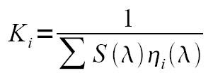
ρ(λ) and S(λ) are the reflectance and light source, respectively and, η(λ) are the spectral sensitivities of the camera (subscripts indicate the channel sensitivity - red, green and blue). K_i are called the white balancing constants of the form:

These constants are important so that the camera renders the correct reflectance of an object. Digital cameras have this option to change their white balance depending on the current source that illuminates on the object i.e. cloudy, sunny, fluorescent, etc. When the white balance of the camera does not match the light source, what happens is that the reflectance of the object is rendered incorrectly by the camera. In such case, we say that the camera is improperly white balanced. We can readily see this if, for example, we see a known white object as a non-white (bluish probably). When faced with such images, image processing techniques has to be done to correct them.

In this activity, we explore two of the white balancing algorithms used for such images -- the White Patch algorithm and the Gray World algorithm.

Algorithms
White Patch (WP) algorithm is implemented by first finding a patch of a known "white" object in the image. The average RGB values (Rw Gw and Bw) of the entire patch is calculated. All 3 channels in the image is normalized using those average values. Essentially, we force the "white patch" to be white. As such, all the other pixels are affected also.
Gray World (GW) algorithm, on the other hand, has the same implementation as the WP algorithm only that the image is normalized by the average RGB values of the entire image. The algorithm , given an image with a sufficient amount of color variations [1], assumes that the average color of the world is gray - a family of white. In this case, we force the image to have a common gray value. As a result, the effect of the illuminant on the image is removed. The image then becomes white-balanced.

Below are images of a scene under constant lighting environment captured by a Motorola W156 camera phone with different white balancing (WB) settings. Both algorithms were performed in each image.

Fig1. (left column)Images containing different colors under different WB settings of the camera and, white-balanced images using (middle) WP and (right) GW algorithms.

Comparing the raw images from the reconstructed images using either of the algorithms, we see that we have successfully implemented the techniques. The background (which is in actual white) in the raw images initially does not appear white. For example, the background of the image using indoor WB camera settings appears blue but now appears white upon white balancing.
Also, we observe that the both algorithms produces different results - which is expected since they have different implementation. It can be seen that the images produces using GW algorithm is much brighter than that of the WP algorithm. In this case, we can infer that after the GW implementation, a lot of pixel values saturated which means that these pixel values exceed the supposedly maximum value of 1. This is not what we want. Here we see the disadvantages of the the GW algorithm. One is that, the image must satisfy a condition (that it must contain a sufficient amount of color variations) for the GW algorithm to work. Another is that since the algorithm normalizes the image using the average RGB values of the image it is expected that saturation of RGB values will occur.

In this part we now use the two algorithms onto monochromatic images.

Figure 2. Monochromatic images capture using different WB camera settings and the reconstructed images using the two algorithms.

From the figure above, we see that the reconstruction of the images using the WP algorithm is way better than the GW algorithm. Again, we go back to the first condition an image must satisfy for the GW to work. Since the images are monochromatic; that is, they do not contain a variety of colors, GW is not appropriate to use.

Strengths and Weaknesses of Each Algorithm.

From the results obtained, we can pretty much gauge the strengths and weaknesses of each algorithm. The GW algorithm does not need any white patch to reconstruct the image hence it is useful when one does not know anything about the image.
Based on the results, we can infer that WP algorithm can work whether the images are monochromatic or colorful. And algorithm can be generically used for white balancing images. However, this will only work if one knows a "white" object in the image.

In general, GW algorithm is more convenient to use than WP. It is easier to implement since we do not need to find white patches in the image and very handy when dealing with colorful images.

I give myself a grade of 9/10 in this activity since I was able to explain the strengths and limitations of the algorithms.

I thank Orly, Thirdy and Master for useful discussions.
References:
[1]http://scien.stanford.edu/class/psych221/projects/00/trek/GWimages.html

Activity 10: Pre-processing Text

In an image, most often than not we only need a certain part or a certain element -- the region of interest(ROI). It may be an object or a text. Either of the two, we need to perform image processing techniques to extract what we need. In this activity, we exploit these techniques particularly in text retrieval. One of its applications is in handwriting recognition.
In this case, we used a scanned image with texts shown in Fig.1(left) as our raw image.

Figure 1. Raw image used in pre-processing text.

We cropped a portion from Fig.1.(left) to be cleaned. Initially the image is rotated so we have to rotate it back so that image processing will be easier. This was done by taking the Fourier transform(FT) of the cropped image in Fig.1(upper right). The frequencies of rotated horizontal lines manifest as a tilted vertical line in the Fourier space. The angle of the tilt was measured using MSPaint. This angle was used to rotate the image back using mogrify command in Scilab. Alternatively, one can measure the tilt angle using Fig.1(upper left) immediately without performing FT.

Figure 2. Removal of horizontal lines on the selected portion of Fig.1(left).

Now that the image is rotated back, the next step in cleaning the image is to remove the horizontal lines. To do this, we get the FT of the image then remove the frequencies of the horizontal lines and take FT again to obtain the reconstructed image.

• Removal of frequencies: Horizontal lines as explained earlier will manifest its frequencies along the vertical axis of the Fourier domain. Blocking out these frequencies will effectively remove the horizontal lines. We do this by multiplying the FT (Fig.2 upper right) to a mask (Fig. 2 lower left) that will completely block out the frequencies along the vertical axis (excluding the center so as not darken the image).
  

After the multiplication, we now take its FT to obtain a partially cleaned image (without the horizontal lines). The image is shown in Fig.2(lower right). Using this image, we are now ready to separate the region of interest (the text) and the background.

We use a simple technique for the separation process -- thresholding. Below is a comparison between Fig.2(lower right) and the thresholded image.

Figure 3. (left) the pre-cleaned image and (right) a thresholded image of the left.

Here we see a separation of the text and the background. Notice, however, we observe a black line dashing through most of the text due to the horizontal line removal previously done. What we need to do next is to remove this black lines. We then preform a closing of the image using a vertical structuring element. In this case, since the texts in the image are tilted, a 4x2 diagonal was used as a structuring element.

Figure 4. The structuring element used and the resulting image after closing

Here we see that that most of the black lines were removed. This is very promising to see. We have used a proper structuring element for the morphological operation. Also, we see that some letters are distinguishable. In Fig.4, we have labeled the blobs found in the image (indicated by a different gray level) and we indeed see some single-letter blobs. It is also interesting to note that the word'"cable" (encircled) is fairly readable although some words are not like the word "power" which we can blame to the quality of the handwriting i.e. some pen strokes are faint that it disappeared upon thresholding.

One of the problems encountered is that it is hard to reduce the letters into 1 pixel thick. To do this, a erosion process must be done using a 1x2 structuring element. However, some strokes on the letters are thin enough such that they are removed upon erosion which we do not want. Hence this operation was not done. Also, it can be observed that the previous "DESCRIPTION" is now almost unreadable. This has been the trade-off of the operation. Since the "DESCRIPTION" did not have the same problem as the rest of the text (dashed by black lines), performing of the close operation made it worse.

Now, we explore if we can find instances of the word "DESCRIPTION" from the whole image. We do this using the following steps:

Step1: Rotate the image
Step2: Binarize the image
Step3: Create a "DESCRIPTION" pattern with the same font and size as in Fig.1(bottom right).
Step4: Correlate the FT of the binarized image with the FT of the produced pattern.
Step5: FT the result in Step 4.

Below are images as a result of Steps 1-3.

Figure 5. (left) binarized rotated image of Fig.1(left); and (right) the pattern used for word
detection. The pattern has font italized Arial Black with fontsize 9.

We then proceed with Step 4 and 5. Patterns that are the same with Fig.5(right) will have a produce a peak at their location - an indication of high value correlation. Below is the image as a result of Step 4 and 5.

Figure 6. Image as a result of correlation

We observed three peaks in the image which correspond to the word "DESCRIPTION". This can be readily verified in Fig.1 (left).

In this activity, I give myself of 10 for doing the job well.