In first part of this activity, we are tasked to find different modes of images,
Dimensions: 504 x 390
Width: 504
Height: 390
Horizontal Resolution: 72 dpi
Vertical Resolution: 72 dpi
Bit Depth: 24
Width: 504
Height: 390
Horizontal Resolution: 72 dpi
Vertical Resolution: 72 dpi
Bit Depth: 24
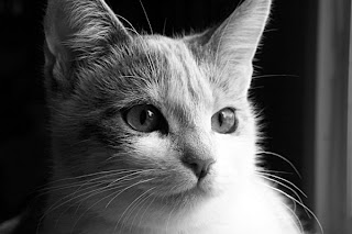
Figure 2. Grayscale image
Dimensions: 600 x 400
Width: 600
Height: 400
Horizontal Resolution: 230 dpi
Vertical Resolution: 230 dpi
Bit Depth: 8
Resolution Unit: 2
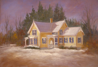
Figure 3. Indexed image
Dimensions: 600 x 410
Width: 600
Height: 410
Bit Depth: 8
Dimensions: 600 x 400
Width: 600
Height: 400
Horizontal Resolution: 230 dpi
Vertical Resolution: 230 dpi
Bit Depth: 8
Resolution Unit: 2

Figure 3. Indexed image
Dimensions: 600 x 410
Width: 600
Height: 410
Bit Depth: 8
Figure 4. Binary image
Dimensions: 600 x 400
Width: 600
Height: 400
Bit Depth: 1
The images were taken from the following sources:
1(left): http://www.thesunblog.com/gourmetgal/fruit.jpg
1(right): http://www.alexmorais.com/Blog%20images/cat-grayscale.jpg
2(left):http://www.gingerbreadartgallery.com/images/archi/large/Gingerbread-house.gif
2(right): http://www.codeproject.com/KB/GDI-plus/AnnotatedImageV2/Mask.png
The binary image was really hard to find.
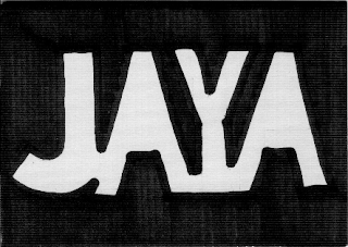
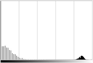
Figure 5. (left) Scanned image and (right)pixel histogram of the image
1(left): http://www.thesunblog.com/gourmetgal/fruit.jpg
1(right): http://www.alexmorais.com/Blog%20images/cat-grayscale.jpg
2(left):http://www.gingerbreadartgallery.com/images/archi/large/Gingerbread-house.gif
2(right): http://www.codeproject.com/KB/GDI-plus/AnnotatedImageV2/Mask.png
The binary image was really hard to find.
For the second part of the activity, a scanned image was used. Here we are tasked to apply thresholding to the image to:
(1) enhance the contrast of the image and
(2) to remove unnecessary pixel values on the region of interest (ROI).
In the figure below, the ROI is the name "JAYA".
(1) enhance the contrast of the image and
(2) to remove unnecessary pixel values on the region of interest (ROI).
In the figure below, the ROI is the name "JAYA".


Figure 5. (left) Scanned image and (right)pixel histogram of the image
Scanned images are usually in RGB mode. In this figure, the mode of the image was changed to grayscale using GIMP. The histogram in Fig.5(left) shows the pixel value distribution on the image (from 0 -255 pixel values). Here we can see the distinct separation between the high value pixels (white) and the low value pixels (black). As such, our ROI is sufficiently separated from the background.
One can also use Scilab to plot the histogram of the image using this code:
g = imread('(path of the image)');
g = int(255*im2gray(g));
[x,y] = size(g);
b = 0:255;
a =[];
for i = 0:255,
a(i+1) = sum((g == i)*1);
end;
plot(b,a/(x*y));
Using this we obtain:
One can also use Scilab to plot the histogram of the image using this code:
g = imread('(path of the image)');
g = int(255*im2gray(g));
[x,y] = size(g);
b = 0:255;
a =[];
for i = 0:255,
a(i+1) = sum((g == i)*1);
end;
plot(b,a/(x*y));
Using this we obtain:
Now, we apply GIMP to threshold the image. In thresholding, we set a certain value (threshold) such that any value less than the threshold will be discarded (pixel value is set to zero when dealing with images) and anything above will be retained or set to a certain value depending on the purpose.
Figure 7. (left) Raw image and (right)the thresholded image
Using a threshold, we are now able to completely separate the ROI from the background.
We can area calculations learned in Activity 2 to Fig.7(right).
We have calculated the area of the ROI in pixels using Green's theorem and pixel counting. Below is the same image with an attached ruler alongside with it. Using this ruler, we can calibrate the pixel-mm ratio which allows us to determine the actual area of the ROI.


nice effort!! :)
ReplyDelete